Getting data in and out of R

One of the great advantages of R is that it recognizes almost any data format that you can throw at it. There are a myriad of different possible file formats but I'll concentrate on the four files that we see almost exclusively in public health: Excel files, Stata .dta files, SAS transport, and sas7bdat files. Luckily, there are a few packages that can help to import and export these files.

First off, I recommend always setting your working directory. This means that you set up to which folder all data is coming in and out of and that way you won't mess up with typing in the directories over and over again. You do it this way:

setwd("C:/Projects/Rforpublichealth")

Great, now that that is done, you can start importing and exporting:

(1) Excel files

This is the easiest one - R has built in functions called read.csv() and write.csv() that work great. They maintain first line variable headings. I find that if you have an .xls file, the best thing to do is to save it as a .csv before trying to input into R.  There are ways to get .xls into R but it's not worth the trouble since converting to a .csv takes 5 seconds.  The function looks like this:

mydata<-read.csv(file="mydata.csv")

There are options for not maintaing first line variable headings (Header=FALSE), but I can't really think of a time that you would want to do that.  You can also change what symbol is delimiting your data (tab delimited for example with sep = "\t") , but again I have never used those options.  If you're in need of those options, you can read about them here.






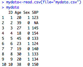
As you see on the left, R will automatically convert missing cells to NA, meaning that it's a numeric variable. If you have periods or something else that indicates missing in your CSV file, you could do a find and replace of the csv file for periods and change them to blanks.






Otherwise you can fix it with an ifelse() statement like:

mydata$SBP<-as.numeric(ifelse(mydata$SBP==".", NA, mydata$SBP))

Or with an apply() statement. Check out my earlier blog post about this.

Back to importing:  If you get an error like the one you see to the right, 99.9% of the time you have misspelled the name of the file or put it into the wrong folder. Always check to make sure the directory name and the file name match up and all your slashes are in the right place.


Now, let's say you change some things and want to export your data back into a csv. To export, you do:

write.csv(mydata, file="mynewcsvfile.csv")


(2) Stata .dta files

For this, you will need the foreign package.  You must first install the foreign package (you just use the menu bar in R, find the "Install packages" option and go from there).  Then you must then load the library this way:

library(foreign)

Now you can use the read.dta() and write.dta() functions. They are very similar to the read and write csv functions, and look like this:

mystatadata<-read.dta(file="mystatafile.dta")

write.dta(mystatadata, file="mystatafile2.dta")


(3) SAS files

(a) SAS transport files

SAS can be tricky because it uses both transport (XPORT) files as well as sas7bdat files and they are very different in terms of their encoding.  The XPORT files are most common and easier to work with.  For these, you need to first install and load the SASxport library

library(SASxport)

Now, you can use the read.xport() function in the same way we have used the other read functions:

mysasdata<-read.xport(file="mysasfile.xpt")

And again we can export:

write.xport(mydata, file="mynewsasfile.xpt")

(b) SAS7bdat files

This used to be a huge pain. Fortunately, there is a new package for reading these files into R called the sas7bat package. First, install this package and load. Then use the read.sas7bdat() function:

library(sas7bdat)

mysas7bdat<-read.sas7bdat(file="myothersasfile.sas7bdat")

However, I have personally had some problems with this function not working for me. Hopefully it will work for you. If it doesn't, you can try to convert the SAS file using StatTransfer or with JMP if you don't have SAS on your computer.

What a nice looking scatterplot!

This week, we look at plotting data using scatterplots. I'll definitely have a post on other ways of plotting data, like boxplots or histograms.

Our data from last week remains the same:

First, a quick way to look at all of your continuous variables at once is just to do a plot command of your data.  Here, I will subset the data to just take three columns and plot those against each other:

plot(mydata[,c(2,4,5)])

This takes all rows, and the columns 2, 4, and 5 from the dataset and plots them all against each other, like this:

Next, I want to make a nice scatterplot of Weight on Height.  The basic format is

plot(xvariable, yvariable)

So it looks like this:

plot(mydata$Weight, mydata$Height)

But this is a little ugly.  Fortunately, there are a million options that I can take advantage of.  In this first post on plotting, I will:

• add labels for the x and y axes (xlab and ylab, respectively) 
• change the dimensions of the plot so it's not quite so condensed (xlim and ylim)
• add a title (main) and change the font size of the title (cex.main)
• get rid of the frame around the plot (frame.plot=FALSE)
• change the type of plotting symbol from little circles to little trianges (pch=2) and make those little triangles blue (col="blue").

plot(mydata$Weight, mydata$Height, xlab="Weight (lbs)", ylab="Height (inches)", xlim=c(80,200), ylim=c(55,75), main="Height vs Weight", pch=2, cex.main=1.5, frame.plot=FALSE , col="blue")

Now, let's get a little more complicated.  I want the color of the plot symbol to be indicative of whether the observation is male or female, and to put a legend in there too. This is super easy right inside the plot function call using the ifelse() statement.  To review, the ifelse() statement is similar to the cond() statement in Stata.  It looks like this:

ifelse(condition, result if condition is true, result if condition is false)

So here I change my parameter col=blue to col=ifelse(mydata$Sex==1, "red", "blue"). This is saying that if the sex is a 1, make the color of the triangle red, else make it blue:

plot(mydata$Weight, mydata$Height, xlab="Weight (lbs)", ylab="Height (inches)", xlim=c(80,200), ylim=c(55,75), main="Height vs Weight", pch=2, cex.main=1.5, frame.plot=FALSE, col=ifelse(mydata$Sex==1, "red", "blue"))

Then I add in the legend. The first two parameters of the legend function are the x and y points where the legend should begin (here at the point (80,75)).  Then I indicate that I want two triangle symbols (pch=c(2,2)).  The first 2 is for the number of symbols and the second 2 is to indicate that pch=2 (a triangle) as it was in the previous example.  Next I say I want the first triangle to be red and the second one blue.  I label the two symbols with the labels "Male" and "Female".  Next, I indicate I want a box around the legend (bty="o") and that I want the box to be darkgreen.  Finally, I indicate that the font size of the whole legend text should be .8. (cex=.8).

legend(80, 75, pch=c(2,2), col=c("red", "blue"), c("Male", "Female"), bty="o",  box.col="darkgreen", cex=.8)

Incidentally, I could get the same plot by identifying "topleft" in my legend() call, as below.  But sometimes it's nice to put the legend exactly where you want it and the legend options only allow for “bottomright”, “bottom”, “bottomleft”, “left”, “topleft”, “top”, “topright”, “right”, “center”.

legend("topleft", pch=c(2,2), col=c("red", "blue"), c("Male", "Female"), bty="o", cex=.8, box.col="darkgreen")

Finally, one of the really nice aspects of R is being able to manipulate the plot region and make it do exactly what you want.  For starters, we can have two plots side by side, by indicating:

par(mfrow=c(1,2))

meaning one row and two columns. If I wanted a 2 by 2 plot area, I would do mfrow=c(2,2).

Now I'll show the full code for the plot below.  The first part is just the first plot we already did, but I add in a vertical line at the average weight and add in text.  The second plot is Height on Age, and I add in the linear regression line.  To do this is quite easy.  I start by running the regression of Height on Age and save it as "reg".  Then I use abline() to add the line to the plot.  Finally, I use the text() function to add text to the plot anywhere I want.  I walk you through the code below:

##set up the plot area with 1 row and 2 columns of plots
par(mfrow=c(1,2))

##first plot height on weight
plot(mydata$Weight, mydata$Height, xlab="Weight (lbs)", ylab="Height (inches)", xlim=c(80,200), ylim=c(55,75), main="Height vs Weight", pch=2, cex.main=1.5, frame.plot=FALSE, col="blue")

##add in the vertical line at the mean of the weight, using na.rm=TRUE to remove the NAs from consideration
abline(v=mean(mydata$Weight, na.rm=TRUE), col="orange")

##add in text at the point (140, 73), with font size .8. The position is 4, meaning that the text moves to the right from the starting point. The "\n" is a carriage return (moves the text to the next line)
text(140,73, cex=.8, pos=4, "Orange line is\n sample average\n weight")

##add in the second plot of height on age
plot(mydata$Age, mydata$Height, xlab="Age (years)", ylab="Height (inches)", xlim=c(0,80), ylim=c(55,75), main="Height vs Age", pch=3, cex.main=1.5, frame.plot=FALSE, col="darkred")


##run a linear regression of Height on Age - if this is confusing, I'll do a post on linear regressions very soon
reg<-lm(Height~Age, data=mydata)

##add the regression line to the plot
abline(reg)


##add text to the plot. Start at the point 0,70.  Position the text to the right of this point (pos=4), make the font smaller (cex=.8), and add in the text using the paste function since I'm pasting in both text and the contents of some variables. For the text, I extract the intercept by taking the first coefficient from the reg object with the code reg$coef[1]; and the coefficient on Age by taking the second coefficient, reg$coef[2].  I round both of those to the second decimal point using round(x,2). There's a lot going on here but hopefully I've unpacked it for everyone.
text(0,72, paste("Height ~ ", round(reg$coef[1],2), "+", round(reg$coef[2],2), "*Age"), pos=4, cex=.8)

Plots are really fun to do in R.  This post was just a basic introduction and more will come on the many other interesting plotting features one can take advantage of in R.  If you want to see more options in R plotting, you can always look at R documentation, or other R blogs and help pages.  Here are a few:

• Graphical parameters explanations
• Stack Overflow has a million questions that have already been asked (or you can ask a new one)
• And to inspire yourself, check out the amazing R Graph Gallery!

Summarizing Data

In this post, I'll go over four functions that you can use to nicely summarize your data.  Before any regression analysis, a descriptive analysis is key to understanding your variables and the relationships between them.  Next week, I'll have a post on plotting, so this post is limited to the summary(), table(), and aggregate() functions.

Here is my dataset for this example:

The first thing I want to do is look at my data overall - get the range of values for each variable, and see what missing values I have.  I can do this simply by doing:

summary(mydata)

This produces the output below, and shows me that both Weight and Height have missing values. The Migrantstatus variable is a factor (categorical), so it lists the number in each category.







If I want to just summarize one variable, I can do summary(mydata$Weight) for example. And remember from last week, that if I just want to summarize some portion of my data, I can subset using indexing like so:  summary(mydata[,c(2:5)])

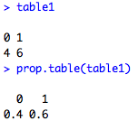
Next, I want to tabulate my data.  I can do univariate and bivariate tables (I can even do more dimensions than that!) by using the table() function.  Table() gives me the totals in each group.  If I want proportions instead of totals, I can use prop.table() around my table() function.  The code looks like this with the output below:

table1<-table(mydata$Sex)

table1
prop.table(table1)



Next, I do the bivariate tables.  The first variable is the row and the second is the column.  I can do proportions here as well, but I must be careful about the margin.  Margin=1 means that R calculates the proportions across rows, while margin=2 is down columns. I show a table of Sex vs Marital status below with two types of proportion tables.

table2<-table(mydata$Sex, mydata$Married)

table2
prop.table(table2, margin=1)
prop.table(table2, margin=2)

And if I want to do three dimensions, I put all three variables in my table() function.  R will give me the 2x2 table of sex and marital status, stratified by the third variable, migrant status.

table3<-table(mydata$Sex, mydata$Married, mydata$Migrantstatus)

The great part about R is that I can take any component of this table that I want.  For example, if I just want the table for migrants, I can do:

table3[,,1]

which tells R to give me all rows and columns, but only for the first category of the third variable.  I get the following output, which you can see is the same as the first part of table 3 from above.

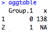
Finally, what if I want to calculate the mean of one variable by another variable? One way to do this is to use the aggregate() function.  Aggregate does exactly that: it takes one variable (the first argument) and calculates some kind of function on it (the FUN= argument), by another variable (the by=list() argument).  So here I am going to do the mean weight for each sex.  Here the syntax is a little funny because R wants a list for the by variable.  I will go over lists at another post in the future, or you can look it up on another R site.

aggtable<-aggregate(mydata$Weight, by=list(mydata$Sex), FUN=mean)
aggtable




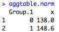
However, something is wrong. The NA in the weight column is messing up my mean calculation.  To get around this, I use the na.rm=TRUE parameter which removes any NAs from consideration.

aggtable.narm<-aggregate(mydata$Weight, by=list(mydata$Sex), FUN=mean, na.rm=TRUE)
aggtable.narm

Victory! If I want to name my columns of this table, I can do:

names(aggtable.narm)<-c("Sex","Meanweight")

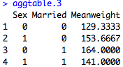
And of course if you want to do mean tables by more than one variable, you can put the all in the list argument, like so: by=list(mydata$Sex, mydata$Married).  The code and output would look like this:


aggtable.3<-aggregate(mydata$Weight, by=list(mydata$Sex, mydata$Married), FUN=mean, na.rm=TRUE)

names(aggtable.3)<-c("Sex","Married","Meanweight")

aggtable.3

Quick and Easy Subsetting

Public health datasets can be enormous and difficult to look at.  Often it is great to be able to only look at specific parts of the dataset, or to only run analysis on a specific part of a dataset.  There are two ways that you can subset a dataset in R:

1. Using the subset() function
2. Using matrix indexing

The first way may sound easier, but the second one is very useful.  Let me show you why.

Let's start with the subset() function.  The basic structure is like this:

subset(x, condition, select=c(var1, var2))

where x is the original dataset you want to subset, condition is a condition on your rows, and select is the columns you want to keep.  So for example, I have a dataset called mydata, shown below.  I want to look at only women that are over 50 years old, and I only want to look at their ID, age, and weight.  Therefore I do this:

sub.data<-subset(mydata, Age>50 & Sex==0, select=c(ID, Age, Weight))

So here I am saying, take the dataset called "mydata", take only rows where the Age >50 and the Sex ==0 (when you write a condition, you always use two equal signs), and then take only the columns ID, Age, and Weight.

Here are the original (left) and the subsetted (right) datasets:

         

You can also do a statement like this:

sub.data2<-subset(mydata, Age>50 & Sex==0, select=c(ID:Sex))

which takes all of the columns between (and including) ID and Sex.  This is nice so you don't have to list out all the variables one by one.

However, now let's take a more real example.  I have a dataset with 200 columns and 3000 rows. I want to keep say 50 columns, but they're not all sequential.  Some are at the beginning of my dataset, some are at the end.  Do I have to go in and write out each name of the variable? Nope.  Instead we can use R's matrix indexing capability.  It's super easy and it goes like this in a general form:

newdata<-originaldata[rows I want, columns I want]

The comma is crucial here since the dataset is organized by rows and columns.  If you don't put anything in the "rows I want" place, R keeps everything. So, for example, I can do this:

sub.data3<-mydata[,c(1:3)]

So this is saying, take the dataset "mydata", and take all the rows (since there is nothing before the comma), and take columns 1-3.  Call this subsetted dataset "sub.data3".  

I can also make the equivalent statement from sub.data2 using indexing like this:

sub.data4<-mydata[mydata$Age>50 & mydata$Sex==0, c(1:3)]

Or, if I just want to look at the first 50 observations and all columns, I can do this:

sub.data5<-mydata[c(1:50), ]

Finally, I can do what I said before, in that I can choose the variables I want from a super long list. I first can find out the index numbers of my columns using the names() command like this:

names(mydata)

Then I can say I want columns 1-5, 8, 12-15, 100-120, 197, and 199.  I can easily do this by saying

sub.data6<-mydata[,c(1:5, 8, 12:15, 100:120, 197, 199)]

Finally, the last thing I want to point out is that if you want to keep most columns but just take away, say, the last 10, you can do this:

sub.data6<-mydata[,-c(190:200)]

The negative sign is like a 'drop' command.  Keep everything except the columns I list out.

It's a very nice feature and very fast!

From continuous to categorical

During data analysis, it is often super useful to turn continuous variables into categorical ones.  In Stata you would do something like this:

gen catvar=0
replace catvar=1 if contvar>0 & contvar<=3
replace catvar=2 if contvar>3 & contvar<=5 

etc.  And then you would label your values like so:

label define agelabel 0 "0" 1 "1-3" 2 "3-5"
label values catvar agelabel

How can we do this in R? There's a great function in R called cut() that does everything at once.  It takes in a continuous variable and returns a factor (which is an ordered or unordered categorical variable).  Factor variables are extremely useful for regression because they can be treated as dummy variables.  I'll have another post on the merits of factor variables soon.

But for now, let's focus on getting our categorical variable.  Here is our data:

And now we want to take that "Age" variable and turn in into a categorical variable.  The most basic statement is like so:


mydata$Agecat1<-cut(mydata$Age, c(0,5,10,15,20,25,30))

Here the function cut() takes in as the first argument the continuous variable mydata$Age and it cuts it into chunks that are described in the second argument.  So here I've indicated to make groups that go from 0-5, 6-10, 11-15, 16-20, etc.  By default, the right side of the interval is closed while the left is open.  You can change that, as we will see below.  First, the output with the new "Agecat" variable:

Now we can customize our intervals.  First, in Agecat2, I show how instead of spelling out every cutoff of the interval, I can just specify a sequence using seq(0, 30, 5) - this means we start at 0 and go to 30 by intervals of 5.

For Agecat3, I switch the default closed interval to be the left one by specifying "right=FALSE".

Finally, for Agecat4 I add in my own labels instead of the default "(0,5]" labels that are provided by R.  I want them to be numbers instead so I indicate "labels=c(1:6)".  The output of all of the options are shown below.

mydata$Agecat2<-cut(mydata$Age, seq(0,30,5))

mydata$Agecat3<-cut(mydata$Age, seq(0,30,5), right=FALSE)

mydata$Agecat4<-cut(mydata$Age, seq(0,30,5), right=FALSE, labels=c(1:6))

Now, if I want some summary statistics or a bivariate table, I get some nice output:



summary(mydata$Agecat1)

  (0,5]  (5,10] (10,15] (15,20] (20,25] (25,30] 
      0       1       2       0       0       1 




table(mydata$Agecat1, mydata$Sex)
       
          0 1
  (0,5]   0 0
  (5,10]  0 1
  (10,15] 1 1
  (15,20] 0 0
  (20,25] 0 0
  (25,30] 0 1

The infamous apply function

For R beginners, the apply() function seems like a secret doorway into programming bliss. It seems so powerful, and yet, beyond reach. For those just starting out, examples of how to use apply() can really help with the intuition of how to harness its power. Here are some great ways to use apply() that can really help make R programming enjoyable and useful.  

First, the general structure of apply() is like so:

apply(x, MARGIN, FUN)

1. The first argument, "x", is whatever dataset or columns of a dataset you want to do something to.
2. The second argument, "MARGIN", is how you want to apply function.  The choices are either over the rows (MARGIN=1) or the columns (MARGIN=2).
3. The third argument (FUN) is the function you apply.  

So for an easy example, if you want to just sum the entries of all the columns in your dataset called "mydata", you can do it this way:

apply(mydata, 2, sum)

But this is not always very useful.  We have other columns in our datasets, and we probably don't want to just sum all the time.  What else can we do? Here are two nice ways to use apply():


1. Counting how many columns meet a certain condition 

I have 13 child outcomes in a dataset named "births" and I want to count up how many live births there were. My "births" data looks like this: 

How can I add up the live births, especially with those pesky NA's in there? Here's a one line way to do it: 

 births$childcount<-apply(births[,1:5], MARGIN=1, function(x) {sum(x=="live birth", na.rm=TRUE)}) 

This code is saying, for the first 5 columns of my dataset births, for each row (MARGIN=1), apply the following function. The function takes x as the input (x is just the births[,1:5] dataset), and sums up for each column of this dataset the number of times it sees "live birth". The na.rm option removes any NA's from consideration.  If you had other conditions, you could say function(x) {sum(x>2010, na.rm=TRUE)}) for example, if you wanted to count up how many years were after 2010. 


 2. Changing coded missing values to NA for multiple columns at a time 

 Often datasets code their missing values as 99 or -99 instead of just leaving them blank. We might want to change these to actual missing so we can work with the data better.  For one variable at at time, I can do it with with ifelse() statement:

originaldata$variable1<-ifelse(originaldata$variable1==99 | originaldata$variable1==-99, NA, originalvariable1)

This is equivalent to the cond() command in stata, where the first argument evaluates the condition, the second argument is what is done if the condition is true, and the third argument is what is done if the condition is false.  

But what if I have 3 or 30 columns that I want to do this to? I don't have to write ifelse() statements for them all individually.  Instead, I use apply.

Here we have a dataset called "originaldata" and we have 4 variables that we want to change from the original missing values to NA values. These variables are in column numbers 2, 4, 5, and 6, as below:

I take the columns of original dataset, and for each of those columns, I use an ifelse statement to check the value of the entry: if it's 99 or -99 I change it to NA, and if it's not then I leave it the way it is. This creates a new dataset called "new data" with just those columns that I choose.

newdata<-apply(originaldata[,c(2,4:6)], MARGIN=2, function(x) {ifelse(x==99 | x==-99, NA,x)})

We print out newdata:

Now if we want the original dataset together with the changed variables, we can just cbind (column bind) them together like so:

alldata<-cbind(originaldata[, c(-2,-4:-6)], newdata)

If you want to be extra fancy, you can just combine the cbind() statement with the apply() in one statement, like this:


newdata<-cbind(originaldata[,c(-2,-4,-6)], apply(originaldata[,c(2,4:6)], MARGIN=2, function(x) {ifelse(x==99 | x==-99, NA,x)}))