Sample size calculations equivalent to Stata functions

========================================================

Hi everyone, I’m trying out R knitr for my blog posts now; let me know what you think!

Recently, I was looking for sample size calculations in R and found that R really doesn’t have good built in funtions for sample size and power. For example, for finding the sample size necessary to find a difference in two proportions, one can use the power.prop.test() function and get the following output:

power.prop.test(n=NULL, .10, .25, .05, .90, alternative="two.sided")

## 
##      Two-sample comparison of proportions power calculation 
## 
##               n = 132.7557
##              p1 = 0.1
##              p2 = 0.25
##       sig.level = 0.05
##           power = 0.9
##     alternative = two.sided
## 
## NOTE: n is number in *each* group

But there are very few options in this function; for example, there is no option for a continuity correction for the normal approximation to binary data, you can’t compare a one sample of a null vs alternative value instead of two sample proportion, and you can’t change the ratio of the size of the two samples. Even more importantly, there’s no way to find effective sample size when data is clustered. There are other functions in R but I found them complicated and not user friendly. The sampsi and sampclus functions in Stata are intuitive and useful, and have all of those important options. I decided to build my own R functions that had the same capabilities, and I’ve posted them here for others to use and comment on. Eventually I would like to make an R package that includes all of these functions for ease of use.

The first function, sampsi.prop(), calculates sample size for one and two sample tests of proportions. The required n for both are as follows: * Two-sample test of equality of proportions, with continuity correction:

\[n_1 = \frac{n'}{4}\left(1+\left\{1+\frac{2(r+1)}{n'r|p_1-p_2|}\right\}^{1/2}\right)^2\]

and \(n_2 = rn_1\)

\[n' = \frac{\left(z_{1-\alpha/2}\left\{(r+1)\bar{p}\bar{q}\right\}^{1/2}+z_{1-\beta}(rp_1q_1+p_2q_2)^{1/2}\right)^2}{r(p_1-p_2)^2}\]

and \(\bar{p} = (p_1+rp_2)/(r+1)\) and \(\bar{q}=1-\bar{p}\)

so that \(n_1=n'\) and \(n_2=rn_1\)

• One-sample test of proportions where null is \(p=p_0\) and alternative is \(p=p_A\):

\[n = \left(\frac{z_{1-\alpha/2}\left\{p_0(1-p_0)\right\}^{1/2} + z_{1-\beta}\left\{p_A(1-p_A)\right\}^{1/2}}{p_A-p_0}\right)^2\]

The function sampsi.prop() takes arguments p1 and p2, which are either the null and alternative proportions, respectively, for the one-sample test, or two proportions for the two-sample test. These arguments are required for the function to run. The rest of the arguments have preset default values so do not need to be indicated, and include the ratio of smaller group to larger group (default=1), power (default of \(\beta=.80\)), significance level (default of \(\alpha=.05\)), a logical argument for whether to include the continuity correction (default is true), whether to perform a two-sided test or one-sided (default is two), and whether to perform the two-sample or one-sample test (defaut is two-sample test). The output is a list object.

sampsi.prop<-function(p1, p2, ratio=1, power=.90, alpha=.05, cont.corr=TRUE, two.sided=TRUE, one.sample=FALSE){
  
  effect.size<-abs(p2-p1)
  avg.p<-(p1+ratio*p2)/(ratio+1)
  sd=ifelse(one.sample==FALSE, sqrt(ratio*p1*(1-p1)+p2*(1-p2)), sqrt(p2*(1-p2)))
  
  z.pow<-qt(1-power, df=Inf, lower.tail=FALSE)
  z.alph<-ifelse(two.sided==TRUE, qt(alpha/2, df=Inf, lower.tail=FALSE), qt(alpha, df=Inf, lower.tail=FALSE))
  ct<-(z.pow+z.alph)
  
  n1<-(z.alph*sqrt((ratio+1)*avg.p*(1-avg.p))+z.pow*sd)^2/(effect.size^2*ratio)
  n1.cont<-ifelse(cont.corr==FALSE, n1, (n1/4)*(1+sqrt(1+(2*(ratio+1))/(n1*ratio*effect.size)))^2)

  n<-(((z.alph*sqrt(p1*(1-p1)))+z.pow*sd)/effect.size)^2
  
  if(one.sample==FALSE){
    col1<-c("alpha", "power", "p1", "p2", "effect size", "n2/n1", "n1", "n2")
    col2<-c(alpha,  power, p1, p2, effect.size, ratio, ceiling(n1.cont), ceiling(n1.cont*ratio))
  }
  else{
    col1<-c("alpha", "power", "p", "alternative", "n")
    col2<-c(alpha, power, p1, p2, ceiling(n))
  }
  ret<-as.data.frame(cbind(col1, col2))
  ret$col2<-as.numeric(as.character(ret$col2))
  colnames(ret)<-c("Assumptions", "Value")
  
  description<-paste(ifelse(one.sample==FALSE, "Two-sample", "One-sample"), ifelse(two.sided==TRUE, "two-sided", "one-sided"), "test of proportions", ifelse(cont.corr==FALSE, "without", "with"), "continuity correction")
  
  retlist<-list(description, ret)
  
  return(retlist)
}

Now we can do the following sample size calculations that match up perfectly to the corresponding commands in Stata:

sampsi.prop(.10, .25)

## [[1]]
## [1] "Two-sample two-sided test of proportions with continuity correction"
## 
## [[2]]
##   Assumptions  Value
## 1       alpha   0.05
## 2       power   0.90
## 3          p1   0.10
## 4          p2   0.25
## 5 effect size   0.15
## 6       n2/n1   1.00
## 7          n1 146.00
## 8          n2 146.00

Notice that the results from the calculation above are corrected for continuity, so do not match up with the power.prop.test output from above. To get those results, specify cont.corr=FALSE like so:

sampsi.prop(.10, .25,  cont.corr=FALSE)

## [[1]]
## [1] "Two-sample two-sided test of proportions without continuity correction"
## 
## [[2]]
##   Assumptions  Value
## 1       alpha   0.05
## 2       power   0.90
## 3          p1   0.10
## 4          p2   0.25
## 5 effect size   0.15
## 6       n2/n1   1.00
## 7          n1 133.00
## 8          n2 133.00

Here are a couple more examples with some of the other defaults changed:

sampsi.prop(.5, .55, power=.8, one.sample=TRUE)

## [[1]]
## [1] "One-sample two-sided test of proportions with continuity correction"
## 
## [[2]]
##   Assumptions  Value
## 1       alpha   0.05
## 2       power   0.80
## 3           p   0.50
## 4 alternative   0.55
## 5           n 783.00

sampsi.prop(.5, .55, ratio=2, two.sided=FALSE)

## [[1]]
## [1] "Two-sample one-sided test of proportions with continuity correction"
## 
## [[2]]
##   Assumptions   Value
## 1       alpha    0.05
## 2       power    0.90
## 3          p1    0.50
## 4          p2    0.55
## 5 effect size    0.05
## 6       n2/n1    2.00
## 7          n1 1310.00
## 8          n2 2619.00

Next we can calculate sample size for a comparison of means. The required n for the one sample and two sample tests are as follows:

• One sample test of mean where null hypothesis is \(\mu=\mu_0\) and the alternative is \(\mu=\mu_A\): \[n = \left\{\frac{(z_{1-\alpha/2} + z_{1-\beta})\sigma}{\mu_A-\mu_0}\right\}^2\]

• Two-sample test of equality of means:

\[n_1 = \frac{(\sigma_1^2+\sigma_2^2/r)(z_{1-\alpha/2}+z_{1-\beta})^2}{(\mu_1-\mu_2)^2}\] \[n_2=rn_1\]

The sampsi.means() function again works the same way as in Stata where you must input as arguments either a null mean and alternative mean for a one-sample test or two means for a two-sample test. At least one standard deviation of the mean is also required. It is possible to have different standard deviations for the two-sample test, but if only the first standard deviation value is assigned and a two-sample test is designated, then the function assumes both standard deviations to be the same. The other arguments and their defaults are similar to the sampsi.prop() function from above.

sampsi.means<-function(m1, m2, sd1, sd2=NA, ratio=1, power=.90, alpha=.05, two.sided=TRUE, one.sample=FALSE){
  
  effect.size<-abs(m2-m1)
  sd2<-ifelse(!is.na(sd2), sd2, sd1)
  
  z.pow<-qt(1-power, df=Inf, lower.tail=FALSE)
  z.alph<-ifelse(two.sided==TRUE, qt(alpha/2, df=Inf, lower.tail=FALSE), qt(alpha, df=Inf, lower.tail=FALSE))
  ct<-(z.pow+z.alph)
  
  n1<-(sd1^2+(sd2^2)/ratio)*(ct)^2/(effect.size^2)
  n<-(ct*sd1/effect.size)^2
  
  if(one.sample==FALSE){
    col1<-c("alpha", "power", "m1", "m2", "sd1", "sd2", "effect size", "n2/n1", "n1", "n2")
    col2<-c(alpha,  power, m1, m2, sd1, sd2, effect.size, ratio, ceiling(n1), ceiling(n1*ratio))
  }
  else{
    col1<-c("alpha", "power", "null", "alternative", "n")
    col2<-c(alpha, power, m1, m2, ceiling(n))
  }
  ret<-as.data.frame(cbind(col1, col2))
  ret$col2<-as.numeric(as.character(ret$col2))
  colnames(ret)<-c("Assumptions", "Value")
  
  description<-paste(ifelse(one.sample==FALSE, "Two-sample", "One-sample"), ifelse(two.sided==TRUE, "two-sided", "one-sided"), "test of means")
  
  retlist<-list(description, ret)
  
  return(retlist)
}

And here are the examples:

sampsi.means(0, 10, sd1=15, power=.8)

## [[1]]
## [1] "Two-sample two-sided test of means"
## 
## [[2]]
##    Assumptions Value
## 1        alpha  0.05
## 2        power  0.80
## 3           m1  0.00
## 4           m2 10.00
## 5          sd1 15.00
## 6          sd2 15.00
## 7  effect size 10.00
## 8        n2/n1  1.00
## 9           n1 36.00
## 10          n2 36.00

sampsi.means(10, 30, sd1=15, sd2=20, alpha=.1, ratio=1)

## [[1]]
## [1] "Two-sample two-sided test of means"
## 
## [[2]]
##    Assumptions Value
## 1        alpha   0.1
## 2        power   0.9
## 3           m1  10.0
## 4           m2  30.0
## 5          sd1  15.0
## 6          sd2  20.0
## 7  effect size  20.0
## 8        n2/n1   1.0
## 9           n1  14.0
## 10          n2  14.0

Finally, we often work with clustered data and would like to calculate sample sizes for clustered observations. Here I created a samp.clus() function that works the same way as the sampclus function in Stata; that is, it takes a sampsi.prop() or sampsi.means() object, along with an interclass correlation coefficient (\(\rho\)) and either the number of observations per cluster or the number of clusters, and calculates the corresponding effective sample size.

samp.clus<-function(sampsi.object, rho, num.clus=NA, obs.clus=NA){
  
  if(is.na(num.clus)&is.na(obs.clus)) print("Either num.clus or obs.clus must be identified")
  else{
    
    so<-sampsi.object[[2]]
    n1<-as.numeric(so[so$Assumptions=="n1",2])
    n2<-as.numeric(so[so$Assumptions=="n2",2])
    
    if(!is.na(obs.clus)){
      deff<-1+(obs.clus-1)*rho
      n1.clus<-n1*deff
      n2.clus<-n2*deff
      num.clus<-ceiling((n1.clus+n2.clus)/obs.clus)
    }
    else if(!is.na(num.clus)){
      
      tot<-(n1*(1-rho)+n2*(1-rho))/(1-(n1*rho/num.clus) - (n2*rho/num.clus))
      if(tot<=0) stop("Number of clusters is too small")
      else{
        obs.clus<-ceiling(tot/num.clus)
        deff<-1+(obs.clus-1)*rho
        n1.clus<-n1*deff
        n2.clus<-n2*deff
      }
    }
    
    col1<-c("n1 uncorrected", "n2 uncorrected", "ICC", "Avg obs/cluster", "Min num clusters", "n1 corrected", "n2 corrected")
    col2<-c(n1, n2, rho, obs.clus, num.clus, ceiling(n1.clus), ceiling(n2.clus))
    ret<-as.data.frame(cbind(col1, col2))
    colnames(ret)<-c("Assumptions", "Value")
    return(ret)
  }
}

Here are a couple of examples of how it works (the same function samp.clus() works for both a sampsi.prop object or a sampsi.means object:

ss<-sampsi.prop(.10, .25, power=.8, two.sided=FALSE)
samp.clus(ss, rho=.05, obs.clus=15)

##        Assumptions Value
## 1   n1 uncorrected    92
## 2   n2 uncorrected    92
## 3              ICC  0.05
## 4  Avg obs/cluster    15
## 5 Min num clusters    21
## 6     n1 corrected   157
## 7     n2 corrected   157

samp.clus(ss, rho=.05, num.clus=150)

##        Assumptions Value
## 1   n1 uncorrected    92
## 2   n2 uncorrected    92
## 3              ICC  0.05
## 4  Avg obs/cluster     2
## 5 Min num clusters   150
## 6     n1 corrected    97
## 7     n2 corrected    97

ss2<-sampsi.means(10, 15, sd1=15, power=.8)
samp.clus(ss2, rho=.05, obs.clus=15)

##        Assumptions Value
## 1   n1 uncorrected   142
## 2   n2 uncorrected   142
## 3              ICC  0.05
## 4  Avg obs/cluster    15
## 5 Min num clusters    33
## 6     n1 corrected   242
## 7     n2 corrected   242

samp.clus(ss2, rho=.05, num.clus=5) 

## Error in samp.clus(ss2, rho = 0.05, num.clus = 5): Number of clusters is too small

##Note: the above won't work because not enough clusters given as input; this error message will occur to warn you. You must increase the number of clusters to avoid the error.

Finally, I add one functionality that Stata doesn’t have with their basic sample size calculations, which is graphing sample size as a function of power. Here, I created two functions for these purposes, for either proprotions or means. The input is the starting point and ending point for the power, as well as the same inputs and defaults from the corresponding sampsi.prop or sampsi.means functions:

graph.power.prop<-function(from.power, to.power,p1, p2, ratio=1, power=.90, alpha=.05, cont.corr=TRUE, two.sided=TRUE, one.sample=FALSE){
  
  seq.p<-seq(from.power, to.power, by=.01)
  n<-rep(NA, length(seq.p))

  for(i in 1:length(seq.p)){
    ob<-sampsi.prop(p1=p1, p2=p2, power=seq.p[i], alpha=alpha, ratio=ratio, cont.corr=cont.corr, two.sided=two.sided, one.sample=one.sample)[[2]]
    n[i]<-as.numeric(ob[7,2])
  }
  plot(n, seq.p, ylab="Power", xlab="n (in smaller arm)", type="l",  main=paste("Power graph for p1=", p1, "and p2=", p2))
}


graph.power.means<-function(from.power, to.power, m1, m2, sd1, sd2=NA, ratio=1, alpha=.05, cont.corr=TRUE, two.sided=TRUE, one.sample=FALSE){
  
  seq.p<-seq(from.power, to.power, by=.01)
  n<-rep(NA, length(seq.p))
  for(i in 1:length(seq.p)){
    ob<-sampsi.means(m1=m1, m2=m2, sd1=sd1, sd2=sd2, power=seq.p[i], alpha=alpha, ratio=ratio,, one.sample=one.sample, two.sided=two.sided)[[2]]
    n[i]<-as.numeric(ob[9,2])
  }
  plot(n, seq.p, ylab="Power", xlab="n (in smaller arm)", type="l",  main=paste("Power graph for m1=", m1, "and m2=", m2))
}

And this is what it looks like. This example will graph power as a function of sample size. We restrict the graph from \(\beta=0.6\) to \(\beta=1\).

graph.power.prop(.6, 1, p1=.20, p2=.35)

Mastering Matrices

R has many ways to store information.  Most of the time, our data comes in the form of a dataset, which we bring into R as a data.frame object. However, there are times when we want to use matrices as well. This post will show you how matrices can be useful and how to manipulate them easily.

First of all, the big difference between matrices and dataframes is that all of the rows and columns of a matrix must have the same class (numeric, character, etc).  In a dataframe, you can have some of each. See my initial post about objects, here.

You can convert from one to the other using as.data.frame() or as.matrix().  Be careful though, that if you convert a dataframe with different classes of columns, then your matrix will just be all character:


In order to have a numeric matrix, I'm going to just take the first 6 columns of the mydata dataframe. I can delete columns of a matrix or dataframe in two ways:

mydata.mat<-as.matrix(mydata[,1:6])
mydata.mat<-as.matrix(mydata[,-7])

These two lines are doing the exact same thing. In the first, I am subsetting the dataframe mydata by taking all rows and the first 6 columns of the dataframe, then I'm converting that subset to a matrix. In the second, I'm taking all rows and all columns except the 7th column. Note that if I wanted to drop even more columns, I would just use the c() function like this:

mydata.mat<-as.matrix(mydata[,c(-3,-7)])

Note now that since I have taken out the one character column in my dataframe before I convert it to a matrix, I will get a numeric matrix instead of a character matrix:

This kind of operation for deleting columns works the same way in both matrices and dataframes. However, to add a column to a dataframe or matrix is different. In a dataframe, you can use the $ operator to identify columns, like mydata$Married is the vector corresponding to the Married column. However, you can't use the $ operator on matrices. You will get the following error that the "$ operator is invalid for atomic vectors", which I see all the time when I'm converting back and forth from dataframes to matrices and make a mistake:

All this message means is that the object you're using is a matrix (mydata.mat) and you can't use the $ operator on a matrix.  If you get this message, you can either use as.data.frame() to convert your matrix to a dataframe, or you can adjust what you are doing to accomodate the rules of matrices.  For adding columns to a matrix, you use cbind(), and likewise for rows, rbind().

So let's say I want to add an age squared column. In the dataframe, I do:

mydata$agesq<-mydata$Age^2

which instantly names the new column "agesq". Now for a matrix, there are two ways to do this, via indexing by number or by name of the original column:

mydata.mat<-cbind(mydata.mat, mydata.mat[,2]^2)
mydata.mat<-cbind(mydata.mat, mydata.mat[,"Age"]^2)

In the first line, I'm taking all rows and the second column of the mydata.mat matrix and squaring it, then I'm column binding it to the original matrix. In the second line, I'm doing the exact same thing, except that instead of indexing with a number, I can use the name of the column "Age". I get the following after running both statements:

Notice that the last two columns of this matrix do not have names, which can be rectified, by using the colnames() function:

colnames(mydata.mat)[7:8]<-c("AgeSq", "AgeSqAgain")

I don't want to rename everything, so I take the 7th and 8th columns and name those appropriately.

Finally, what can matrices do for us? One important aspect of matrices is of course matrix multiplication, which is how we do any multivariable regression analysis. I'll do a post soon on regression analysis by hand in R. But another reason is that matrices are great way to store values that you return during the course of running a loop.

For example, say I want to show how great the central limit theorem is. I'll generate deviates from  some other distribution, say the Poisson, and take the mean of the draws each time. I'll do this 1000 times and then show what the histogram looks like.  In a problem like this, I'll use a loop.  I'll also use a matrix to store the mean each time.

Ok, we start out by initializing a matrix. We'll create a matrix of all NAs with 1000 rows and 3 columns using the matrix() function:

mat1<-matrix(NA, nrow=1000, ncol=3)

Next, we'll set up the for() loop. Let's look at it first and then go through the logic:

for(i in 1:nrow(mat1)){

  vec1<-rpois(1,1)
  vec2<-rpois(10,1)
  vec3<-rpois(100,1)
  mat1[i,]<-c(mean(vec1), mean(vec2), mean(vec3))
 
}

So in the first line, we're saying for each value of i going from i=1 to i=nrow(mat1), do the stuff in the loop. We could have written 1:1000, but it's nice to leave it as nrow(mat1) since we may want to change the size of mat1 later and this way the loop will still be fine.

Next, we draw from a Poisson distribution three times, each time a larger number of draws (first 1 draw, then 10, then 100), and each time with a lambda of 1.

Finally, and this is where the matrix comes in, we'll take the mean of each one of those vectors and store it. We will store the three values in the ith row of the mat1 matrix, filling in all three columns.  In a longer way, I could have done:

mat1[i,1]<-mean(vec1)
mat1[i,2]<-mean(vec2)
mat1[i,3]<-mean(vec3)

and it would have come out the same, but the first way is nicer since it's more compact. Remember that matrices are just columns and rows of vectors, so you can always assign a vector to a row, as long as it's the same length. When you concatenate numbers (using the c() function), you make a vector, which is why it works.

Now, let's see how the old CLT is working by plotting some histograms:

par(mfrow=c(1,3))
hist(mat1[,1], main="n=1")
hist(mat1[,2], main="n=10")
hist(mat1[,3], main="n=100")

Again, with the histograms, I can plot each column at a time by subsetting the mat1 matrix:

Pretty nice! Other very helpful places to better understand matrices:

• UCLA IDRE
• Quick-R

Extracting Information From Objects Using Names()

One of the big differences between a language like Stata compared to R is the ability in R to handle many different types of objects at once, and combine them together or pull them apart.  I had a post about objects last year, but I thought I'd show in this post how to extract information from objects you create in R.

For this example, I'll go back to a dataset I've used in the past called mydata.Rdata and it's in the Code and Data Download site.

One function that is extremely useful to know is names().  The names() function will show you everything that is stored in R under that object name.  So, for example, if you do

where mydata is a dataframe object, you will get the names of the columns, which are the vectors that comprise the dataframe. Note that names(mydata) is an object itself (because everything is an object in R) - it is a character vector of length 7.  You can save this vector and print out the class to verify this.

But names() can be useful for much more than just column names, as we'll see in a moment.

But before we go on, let's take a moment to remember how subsetting works. In subsetting, you use square brackets to pull out exactly the element of an object that you want. So if I want to subset a dataframe, I can say

mydata.subset<-mydata[,c(1:2)]

which is saving into the new object mydata.subset, all the rows and only the first two columns of the mydata dataframe.

Now, let's combine the concept of using the names() function with the concept of subsetting to change one of the column names of our dataset:

names(mydata)[4]<-"Weight_lbs"

Here we are saying, of the names(mydata) object, take the fourth component and make it "Weight_lbs".  Now, if you run the names() on our dataframe, we find the change has been made:




Ok, so now we'll see how the names() function can be used in other applications.

1. Summary objects

There are two ways to extract information from objects in R, using subsetting and using the "$" operator. 

Below, we summarize the Age vector and store the results in sum.vec.  We print out the sum.vec object and the print out the corresponding names.  Now we can extract the 1st element of the summary vector of Age in the following way using the [ ] operator.

This gives us the first element, which is the minimum. We could also do:

sum.vec[c(2,3,5)] 

for the 25th, 50th, and 75th percentiles.


The other way to extract is by using "$".  For example, the summary() function on a table object gives you a Chi squared test:

Here, you can extract any of the pieces of information that came out in the test, including the number of cases, the number of variables, the test statistic, etc.  We can extract the pvalue of the test statistic by using the "$" operator, like this:

Let's see how this can be useful in the next example.

2. Regressions and statistical tests

The standard linear regression that we run in R is using lm().  It looks like this:

But there's a lot more that R has calculated that is not shown here. We can see this by saving this linear regression as an object and running names() on it:

So we see that saved under the reg.object are the coefficients, the residuals, fitted values, degrees of freedom, and a lot more.   To find out everything that names() provides for a given object, look it up by doing ?lm.  Now, to extract any of these components, like the residuals, use the "$" operator like this:

reg.object$residuals

You can make use of this extraction by taking the mean of the residuals

or plotting their distribution:

hist(reg.object$residuals, main="Distribution of Residuals" ,xlab="Residuals")

Don't forget that you can summarize regression objects using summary(), and get the names() of that summary too, like this:

summary(reg.object)
names(summary(reg.object))

which will give you more objects you can extract from your regression. You can use the names() function on any statistical model or function such as aov(), t.test(), chisq.test(), etc.

3.  Histograms and boxplots

Finally, let's go back to that histogram and save that into an object. There are objects under names() of the histogram object now:

I showed how you can manipulate those in my post on histograms.

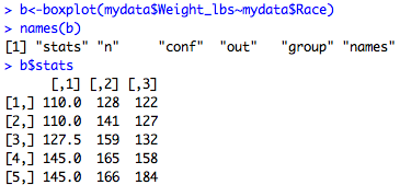
Similarly, for boxplot:













Here I've extracted the stats object which gives you the lower whisker, the lower hinge, the median, the upper hinge, and the upper whisker for each group, which you can see below.

Normal distribution functions

Ah, the Central Limit Theorem.  The basis of much of statistical inference and how we get those 95% confidence intervals.  It's just so beautiful!  Lately, I have found myself looking up the normal distribution functions in R.  They can be difficult to keep straight, so this post will give a succinct overview and show you how they can be useful in your data analysis.

To start, here is a table with all four normal distribution functions and their purpose, syntax, and an example:

	Purpose	Syntax	Example
rnorm	Generates random numbers  from normal distribution	rnorm(n, mean, sd)	rnorm(1000, 3, .25) Generates 1000 numbers from a normal with mean 3 and sd=.25
dnorm	Probability Density Function (PDF)	dnorm(x, mean, sd)	dnorm(0, 0, .5) Gives the density (height of the PDF) of the normal with mean=0 and sd=.5.
pnorm	Cumulative Distribution Function (CDF)	pnorm(q, mean, sd)	pnorm(1.96, 0, 1) Gives the area under the standard normal curve to the left of 1.96, i.e. ~0.975
qnorm	Quantile Function - inverse of pnorm	qnorm(p, mean, sd)	qnorm(0.975, 0, 1) Gives the value at which the CDF of the standard normal is .975, i.e. ~1.96

Note that for all functions, leaving out the mean and standard deviation would result in default values of mean=0 and sd=1, a standard normal distribution.

Another important note for the pnorn() function is the ability to get the right hand probability using the lower.tail=FALSE option.  For example,

In the first line, we are calculating the area to the left of 1.96, while in the second line we are calculating the area to the right of 1.96.

With these functions, I can do some fun plotting. I create a sequence of values from -4 to 4, and then calculate both the standard normal PDF and the CDF of each of those values.  I also generate 1000 random draws from the standard normal distribution. I then plot these next to each other. Whenever you use probability functions, you should, as a habit, remember to set the seed. Setting the seed means locking in the sequence of "random" (they are pseudorandom) numbers that R gives you, so you can reproduce your work later on.

set.seed(3000)
xseq<-seq(-4,4,.01)
densities<-dnorm(xseq, 0,1)
cumulative<-pnorm(xseq, 0, 1)
randomdeviates<-rnorm(1000,0,1)
 
par(mfrow=c(1,3), mar=c(3,4,4,2))

plot(xseq, densities, col="darkgreen",xlab="", ylab="Density", type="l",lwd=2, cex=2, main="PDF of Standard Normal", cex.axis=.8)

plot(xseq, cumulative, col="darkorange", xlab="", ylab="Cumulative Probability",type="l",lwd=2, cex=2, main="CDF of Standard Normal", cex.axis=.8)

hist(randomdeviates, main="Random draws from Std Normal", cex.axis=.8, xlim=c(-4,4))

The par() parameters set up a plotting area of 1 row and 3 columns (mfrow), and move the three plots closer to each other (mar). Here is a good explanation of the plotting area.  The output is below:

Now, when we have our actual data, we can do a visual check of the normality of our outcome variable, which, if we assume a linear relationship with normally distributed errors, should also be normal. Let's make up some data, where I add noise by using rnorm() - here I'm generating the same amount of random numbers as is the length of the xseq vector, with a mean of 0 and a standard deviation of 5.5.

xseq<-seq(-4,4,.01)

y<-2*xseq + rnorm(length(xseq),0,5.5)

And now I can plot a histogram of y (check out my post on histograms if you want more detail) and add a curve() function to the plot using the mean and standard deviation of y as the parameters:

hist(y, prob=TRUE, ylim=c(0,.06), breaks=20)
curve(dnorm(x, mean(y), sd(y)), add=TRUE, col="darkblue", lwd=2)

Here, the curve() function takes as its first parameter a function itself (or an expression) that must be written as some function of x.  Our function here is dnorm(). The x in the dnorm() function is not an object we have created; rather, it's indicating that there's a variable that is being evaluated, and the evaluation is the normal density at the mean of y and standard deviation of y. Make sure to include add=TRUE so that the curve is plotted on the same plot as the histogram.  Here is what we get:

Here are some other good sources on the topic of probability distribution functions:

• Quick-R
• Overview of Normal Distribution in R
• R-Bloggers Introduction
• Probability Distributions in R, UMN
• R Tutor

Converting a dataset from wide to long

I recently had to convert a dataset that I was working with from a wide format to a long format for my analysis.  I struggled with this a bit, but finally found the right sources and the right package to do it, so I thought I'd share my practical example of reshaping data in R. This post is specifically helpful for those using Demographic and Health Survey (DHS) data.

The DHS dataset includes one observation for each woman. For each observation, there are 20 columns for each birth she could have had for 16 different characteristics.  If no birth happened then the cell is left missing. The characteristics include birth month, birth year, sex of the child, death month, death year, who the child lives with, current age of child, and so on.

For clarity, I've shortened the data to just 7 observations and two characteristics of each birth (b2 and b4) for 3 possible births:

Here v012 is the mother's age, all the b2 variables are year of births, and the b4 variables are the sex of the child.

So the first subject, aged 30, has had two births - one in 2000 and one in 2005, both boys.  Since she did not have a third birth yet, her values for b2_03 and b4_03 are missing.

I would like to convert this dataset to one where I have one observation per child born - i.e. from the wide format to the long format. Specifically, I would like the columns to just be the caseid of the mother, age of the mother, year of birth of the child, and sex of the child.

There are a number of ways of doing this in R, including melt() and cast(), plyr(), aggregate(), and others.  However, after a good deal of struggle and looking things up, I found that the reshape() function is the most intuitive and user-friendly for the needs of this problem. You don't need to use melt and cast at all, which are difficult to manipulate in my opinion.

The reshape() function takes in a number of important parameters that will be necessary for our transformation (there are more parameters than this, but I've boiled it down to the ones that are crucial):

reshape(data, varying = NULL, timevar = "time", idvar = "id", direction, sep = "")

where
data = dataframe you want to convert
varying = columns in the wide format that correspond to a single column in the long format
timevar = name of new variable that differentiates multiple observations from the same individual
idvar = variable in your dataset that identifies multiple records from the same individual
direction = "wide" if you're going from long to wide and "long" if you're going from wide to long
sep = the symbol that separates the name of a varying column from its number

Ok, so the most important thing about the reshape function is that you have to give it variable names that it can understand. Specifically, the columns that I want to turn into one column should all follow the same structure in the naming convention. It can be anything with a pattern like this:

Birthyear_1, Birthyear_2, Birthyear_3
b1, b2, b3
year.1, year.2, year.3

etc.  As long as they follow the same text and number pattern. If the dataset is not in this format, you will have a lot of problems and I suggest changing your variable names before trying to convert. For the first example, you would use sep="_", the second would be sep="", and the third is sep="." and all of these are valid.

Ok, so let's try it out. All variables that we want to convert into one column we can put into the varying parameter and R will sort them out based on the naming patterns. We specify a long direction, that our id variable is caseid, and, importantly, that the separating symbol between the name of the variable and its order number is a "_".

births.long1<-reshape(births.wide, varying=c("b2_01","b2_02","b2_03", "b4_01", "b4_02", "b4_03"), direction="long", idvar="caseid", sep="_")

This gives us the following result (truncated picture):

Which is what we wanted! Each observation is now a birth, with corresponding mother caseid and age, and the year (b2) and sex of the child (b4) for each observation correctly lined up. R has added in the time variable which is just the number after the "_" for the varying variables. Notice that R automatically orders the dataset by this time variable, so you will have to re-order if you want it by caseid.

If you wanted to convert all of the 16 characteristics of each birth, you do not need to write out each individual variable. You can easily do it like this, indicating the number of the columns that you want:

births.long2<-reshape(births.wide, varying=c(3:8), direction="long", idvar="caseid", sep="_", timevar="order")

births.long2<-births.long2[order(births.long2$caseid),]

names(births.long2)<-c("subject","age","order", "birthyear", "childsex")

births.long2<-na.omit(births.long2)

Here, I've specified that all variables from column 3 to column 8 are varying variables, and I've also indicated that the new variable that R creates should be called "order" instead of the default "time". Then I reorder my dataset by caseid, name the new columns, and take out all of the missing observations, which are just non-existent births. I get the following result: 

Notice how subject 6 is completely gone because she did not have any children and this is now a dataset of children ever born.

I've made this example of reshape very specific to DHS data, but there are also many great sources on how to reshape data in R. Here are a couple that I found especially helpful:

• TRinker's R Blog
• UCLA R Stats