Data types, part 3: Factors!

In this third part of the data types series, I'll go an important class that I skipped over so far: factors.

Factors are categorical variables that are super useful in summary statistics, plots, and regressions. They basically act like dummy variables that R codes for you.  So, let's start off with some data:

and let's check out what kinds of variables we have:

so we see that Race is a factor variable with three levels.  I can see all the levels this way:


So what his means that R groups statistics by these levels.  Internally, R stores the integer values 1, 2, and 3, and maps the character strings (in alphabetical order, unless I reorder) to these values, i.e. 1=Black, 2=Hispanic, and 3=White.  Now if I were to do a summary of this variable, it shows me the counts for each category, as below.  R won't let me do a mean or any other statistic of a factor variable other than a count, so keep that in mind. But you can always change your factor to be numeric, which I'll go over next week.

If I do a plot of age on race, I get a boxplot from the normal plot command since that is what makes sense for a categorical variable:

plot(mydata$Age~mydata$Race, xlab="Race", ylab="Age", main="Boxplots of Age by Race")

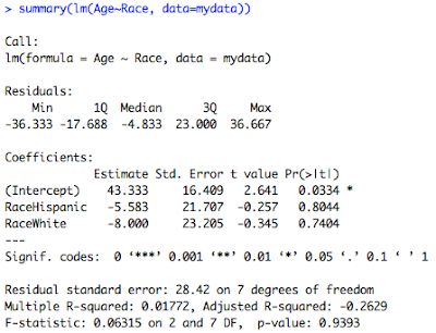
Finally, if I do a regression of age on race, notice how I instantly get dummy variables:

summary(lm(Age~Race, data=mydata))











Here Black is the reference category since it's the first level by alphabetical order.







What if I want to run the same regression as before, but I want to use Hispanic as my reference group?  Very easily, I just relevel the factor like this and get the resulting regression output:

mydata$Race2<-relevel(mydata$Race, "Hispanic")

summary(lm(Age~Race2, data=mydata))

Notice how now the Hispanic category is the reference.




So that is great stuff. But it's really important to know how to manipulate the factor variables. First, I can create factors using the factor() function.  I notice from viewing my dataset above (or from running class(mydata$Marriage)) that marriage is numeric and coded as 0, 1, or 2.  I find out in my codebook that those values correspond to Single, Married, and Divorced/Widowed. We can fix that this way:

mydata$Married.cat<-factor(mydata$Married, labels=c("Single", "Married", "Divorced/Widowed"))

This will create an unordered factor where 1=Single, 2=Married, and 3=Divorced/Widowed.

Now let's say I want to create a variable that describes whether someone's weight is "Low", "Medium", and "High".  In this case, I'll use the cut() function, which instantly creates a factor that I can label, then I use the ordered() function around the cut function to order the levels.  I show it in different colors for ease of viewing the two functions that I'm nesting:

mydata$Weight.type<-ordered(cut(mydata$Weight, c(0,135,165,200), labels=c("Low", "Medium", "High")))


If I print out the class and the contents of the variable (left) , I notice that it's an ordered factor and it tells me that Low<Medium< High, which is what I want.

We can see the new additions to my dataset (I'm showing just the relevant columns):

One caveat with factors - if you start off with a level and then you drop the only observations with that level, R still holds on to the level as a stored value and this can mess up your later analysis.  For example, I subset my data to the first 6 rows so that I eliminate all Hispanic subjects from my data, but R keeps Hispanic as a possible level:


mynewdata<-mydata[1:6,]
summary(mynewdata$Race)






So here Hispanic just has a 0 count, but is still a category.  This can be really annoying, like when you're making a barplot and the category is still showing up in the plot.

One quick way to get rid of this is to use the droplevels() function to drop all unused levels from your dataset. A commentator let me know that this function was introduced in R 2.12.0. Before, it was necessary to use a separate package called gdata. The function takes the whole dataframe as the argument, and you can use the except argument to list the indices of columns that you do not want subject to the dropping:

finaldata<-droplevels(mynewdata)
summary(finaldata$Race)






You could do all this very efficiently in one step like this without changing the name of your dataframe:

mydata<-droplevels(mydata[1:6,])

which is why we love R!