Data types part 4: Logical class

First, an update:  A commentator has asked me to post my code so that it is easier to practice the examples I show here.  It will take me a little bit of time to get all of my code for past posts well-documented and readable, but I have uploaded the code and data for the last 4 posts, including this one, here:

Code and Data download site

Unfortunately, I could not find a way to attach it to blogger, so sorry for the extra step.
_________________________________________________________________________

Ok, now on to Data types part 4: Logical

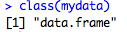
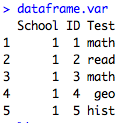
I started this series of posts on data types by saying that when you have a dataframe like this called mydata:




you can't do this in R:

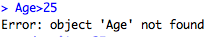
Age<25

Because Age does not exist as an object in R, and you get the error below:

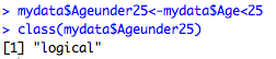
But then what happens when I do,

mydata$Age<25

This is perfectly legal to do in R, but it's not going to drop observations. With this kind of statement, you are asking R to evaluate the logical question "Is it true that mydata$Age is less than 25?".  Well, that depends on which element of the Age vector, of course. Which is why this is what you get when you run that code:



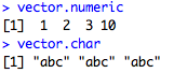
On first glance, this looks like a character vector.  There is a string of entries using character letters after all.  But it's not character class, it's the logical class.  If you save this string of TRUE and FALSE entries into an object and print its class, this is what you get:



The logical class can only take on two values, TRUE or FALSE.  We've seen evaluations of logical operations already, first in subsetting, like this:

mysubset<-mydata[mydata$Age<40,]

Check out my post on subsetting if this syntax is confusing. In a nutshell, R evaluates all rows and keeps only those that meet the criteria, which is only rows where Age has a value of under 40 and all columns.

Or here, in ifelse() statements

mydata$Young<-ifelse(mydata$Age<25,1,0)

More on ifelse() statements here. The ifelse() function is really useful, but is actually overkill when you're just creating a binary variable. This can be done faster by taking advantage of the fact that logical values of TRUE always have a numeric value of 1, while logical values of FALSE always have a numeric value of 0.

That means all I need to do to create a binary variable of under age 25 is to convert my logical mydata$Ageunder25 vector into numeric.  This is very easy with R's as.numeric() function. I do it like this:

mydata$Ageunder25_num<-as.numeric(mydata$Ageunder25)

or directly without that intermediate step like this:

mydata$Ageunder25_num<-as.numeric(mydata$Age<25)

Let's check out the relevant columns in our dataframe:

We can see that the Ageunder25_num variable is an indicator of whether the Age variable is under 25.

Now the really, really useful part of this is that you can use this feature to turn on and off a variable depending on its value. For example, say you got your data and realized that some of the height values were in inches and some were in centimeters, like this:



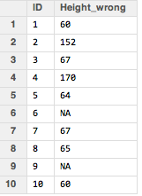
Those heights of 152 and 170 are in centimeters while everything else is inches.  There are various ways to fix it, but one way is to check which values are less than, say 90, which is probably a safe cutoff and create a new column that keeps those values under 90 but converts the values over 90.  We can do this in this way:


mydata$Height_fixed_in<-  as.numeric(mydata$Height_wrong<90)*mydata$Height_wrong 
+ as.numeric(mydata$Height_wrong>=90)*mydata$Height_wrong/2.54

So the first half of the calculation (in red) is "turned on" when Height_wrong is less than 90, because the value of the logical statement is a numeric TRUE, i.e. a 1, and this value of 1 is multiplied by the original Height column.  The second part of the statement (in blue) is FALSE and so is just 0 times something so it's 0.  If the Height_wrong column is greater than 90, then the first half is just 0 and the second half  is turned on and thus the Height_wrong variable is divided by 2.54 cm, converting it into inches. We get the result below:

Another useful way to use the as.numeric() and logical classes to your advantage is a situation like this:

I have in my dataset the age of the last child born (and probably other characteristics of this child not shown), and then just the number of other children for each woman.  I want to get a total number of children variable.  I can do it simply in the following way. 

First, a note about the is.na() function.  If you want to check if a variable is missing in R, you don't use syntax like "if variable==NA" or "if variable==.".  This is not going to indicate a missing value. What you want to use instead is is.na(variable) like this:

is.na(newdata$Child1age)

Which gives you a logical vector that looks like this:

If you want to check if a variable is not missing, you use the ! sign (meaning "Not") in front and check it like this:

We've seen this kind of thing before!  Now we can translate this logical vector into numeric and add it to the number of other children, like this:

newdata$Totalnumchildren<-as.numeric(!is.na(newdata$Child1age))+newdata$Numotherchildren

We get the following:

If we want to get those NAs to be 0, we can again use the is.na() function and replace whereever Totalnumchildren is missing with a 0 like this:

newdata$Totalnumchildren[is.na(newdata$Totalnumchildren)]<-0

Data types, part 3: Factors!

In this third part of the data types series, I'll go an important class that I skipped over so far: factors.

Factors are categorical variables that are super useful in summary statistics, plots, and regressions. They basically act like dummy variables that R codes for you.  So, let's start off with some data:

and let's check out what kinds of variables we have:

so we see that Race is a factor variable with three levels.  I can see all the levels this way:


So what his means that R groups statistics by these levels.  Internally, R stores the integer values 1, 2, and 3, and maps the character strings (in alphabetical order, unless I reorder) to these values, i.e. 1=Black, 2=Hispanic, and 3=White.  Now if I were to do a summary of this variable, it shows me the counts for each category, as below.  R won't let me do a mean or any other statistic of a factor variable other than a count, so keep that in mind. But you can always change your factor to be numeric, which I'll go over next week.

If I do a plot of age on race, I get a boxplot from the normal plot command since that is what makes sense for a categorical variable:

plot(mydata$Age~mydata$Race, xlab="Race", ylab="Age", main="Boxplots of Age by Race")

Finally, if I do a regression of age on race, notice how I instantly get dummy variables:

summary(lm(Age~Race, data=mydata))











Here Black is the reference category since it's the first level by alphabetical order.







What if I want to run the same regression as before, but I want to use Hispanic as my reference group?  Very easily, I just relevel the factor like this and get the resulting regression output:

mydata$Race2<-relevel(mydata$Race, "Hispanic")

summary(lm(Age~Race2, data=mydata))

Notice how now the Hispanic category is the reference.




So that is great stuff. But it's really important to know how to manipulate the factor variables. First, I can create factors using the factor() function.  I notice from viewing my dataset above (or from running class(mydata$Marriage)) that marriage is numeric and coded as 0, 1, or 2.  I find out in my codebook that those values correspond to Single, Married, and Divorced/Widowed. We can fix that this way:

mydata$Married.cat<-factor(mydata$Married, labels=c("Single", "Married", "Divorced/Widowed"))

This will create an unordered factor where 1=Single, 2=Married, and 3=Divorced/Widowed.

Now let's say I want to create a variable that describes whether someone's weight is "Low", "Medium", and "High".  In this case, I'll use the cut() function, which instantly creates a factor that I can label, then I use the ordered() function around the cut function to order the levels.  I show it in different colors for ease of viewing the two functions that I'm nesting:

mydata$Weight.type<-ordered(cut(mydata$Weight, c(0,135,165,200), labels=c("Low", "Medium", "High")))


If I print out the class and the contents of the variable (left) , I notice that it's an ordered factor and it tells me that Low<Medium< High, which is what I want.

We can see the new additions to my dataset (I'm showing just the relevant columns):

One caveat with factors - if you start off with a level and then you drop the only observations with that level, R still holds on to the level as a stored value and this can mess up your later analysis.  For example, I subset my data to the first 6 rows so that I eliminate all Hispanic subjects from my data, but R keeps Hispanic as a possible level:


mynewdata<-mydata[1:6,]
summary(mynewdata$Race)






So here Hispanic just has a 0 count, but is still a category.  This can be really annoying, like when you're making a barplot and the category is still showing up in the plot.

One quick way to get rid of this is to use the droplevels() function to drop all unused levels from your dataset. A commentator let me know that this function was introduced in R 2.12.0. Before, it was necessary to use a separate package called gdata. The function takes the whole dataframe as the argument, and you can use the except argument to list the indices of columns that you do not want subject to the dropping:

finaldata<-droplevels(mynewdata)
summary(finaldata$Race)






You could do all this very efficiently in one step like this without changing the name of your dataframe:

mydata<-droplevels(mydata[1:6,])

which is why we love R!

Data types part 2: Using classes to your advantage

Last week I talked about objects including scalars, vectors, matrices, dataframes, and lists.  This post will show you how to use the objects (and their corresponding classes) you create in R to your advantage.

First off, it's important to remember that columns of dataframes are vectors.  That is, if I have a dataframe called mydata, the columns mydata$Height and mydata$Weight are vectors. Numeric vectors can be multiplied or added together, squared, added or multiplied by a constant, etc. Operations on vectors are done element by element, meaning here row by row.

First, I read in a file of data, called mydata, using the read.csv() function. I get the dataframe below:

I check the classes of my objects using class(), or all at the same time with ls.str().

class(mydata$Weight)
class(mydata$Height)

or

So I see that mydata is a dataframe and all my columns are numeric (num).  Now, if I want to create a new column in my dataset which calculates BMI, I can do some vector operations:

mydata$BMI<-mydata$Weight/(mydata$Height)^2 * 703

Which is the formula for BMI from weight in pounds and height in inches. Notice how if any component of the calculation is a missing (NA) value, R calculates the BMI as NA as well.

Now I can do summary statistics on my data and store those as a matrix. For example, I start with summary statistics on my Age vector:

summary(mydata$Age)






If I want to extract an element of this summary table, say the minimum, I can do

summary(mydata$Age)[1]

which extracts the first element (of 6) of the summary table.

But what I really want is a summary matrix of a bunch of variables: Age, Sex, and BMI.  To do this I can rowbind the summary statistics of those three variables together using the rbind() function, but only take the 1st, 4th, and 6th elements of the summary table, which as you can see correspond to the Min, Mean, and Max. This creates a matrix, which I call summary.matrix:

summary.matrix<-rbind(summary(mydata$Age)[c(1,4,6)], summary(mydata$BMI)[c(1,4,6)], summary(mydata$Sex)[c(1,4,6)])

Rowbinding is basically stacking rows on top of each other.  I add rownames and then print the class of my summary matrix and the results.

rownames(summary.matrix)<-c("Age", "BMI", "Sex")
class(summary.matrix)
summary.matrix










There is also a much more efficient way of doing this using the apply() function.  Previously I had another post on the apply function, but I find that it takes a lot of examples to get comfortable with so here is another application.

Apply() is a great example of classes because it takes in a dataframe as the first argument (mydata, all rows, but I choose only columns 2, 3, and 7).  I then apply it to the numeric vector columns (MARGIN=2) of this subsetted dataframe, and then for each of those columns I perform the mean and standard deviation, removing the NA's from consideration.  I save this in a matrix I call summary.matrix2.

summary.matrix2<-apply(mydata[,c(2,3,7)], MARGIN=2, FUN=function(x) c(mean(x,na.rm=TRUE), sd(x, na.rm=TRUE)))

I then rename the rows of the this matrix and print the results, rounded to two decimal places.  Notice how the format of the final matrix is different here. Above the rows were the variables and the columns the summary statistics, while here it is reversed.  I could have column binded (cbind() instead of the rbind()) in the first case and I would have gotten the matrix transposed to be like this one.

rownames(summary.matrix2)<-c("Mean", "Stdev")
round(summary.matrix2, 2)

Finally, I want to demonstrate how you can take advantage of scalars and vectors when graphing. Creating scalar and vectors objects is really helpful when you are doing the same task multiple times.  I give the example of creating a bunch of scatterplots.

I want to make a scatterplot for each of three variables (Height, Weight, and BMI) against age.  Since all three scatterplots are going to be very similar, I want to standardize all of my plotting arguments including the range of ages, the plot symbols and the plot colors.  I want to include a vertical line for the mean age and a title for each plot.  The code is below:


##Assign numeric vector for the range of x-axis
agelimit<-c(20,80)

##Assign numeric single scalar to plotsymbols and meanage
plotsymbols<-2
meanage<-mean(mydata$Age)

##Assign single character words to plottype and plotcolor 
plottype<-"p"
plotcolor<-"darkgreen"

##Assign a vector of characters to titletext
titletext<-c("Scatterplot", "vs Age")

Ok, so now that I have all those assigned, I can plot the three plots all together using the following code.  Notice how all the highlighted code is the same in each plot (except for the main title) and I'm using the assigned objects I just created.  The great part about this is that if I decide I actually want to plot color to be red, I can change it in just one place.  You can think about how this would be useful in other situations (data cleaning, regressions, etc) when you do the same thing multiple times and then decide to change one little parameter. If you're not sure about the code below, I posted on the basics of plotting here.

##Plot area is 1 row, 3 columns
par(mfrow=c(1,3))

##Plot all three plots using the assigned objects
plot(mydata$Age, mydata$Height, xlab="Age", ylab="Height", xlim=agelimit,pch=plotsymbols, type=plottype, col=plotcolor, main=paste(titletext[1], "Height", titletext[2]))
abline(v=meanage)

plot(mydata$Age, mydata$Weight, xlab="Age", ylab="Weight", xlim=agelimit,pch=plotsymbols, type=plottype, col=plotcolor, main=paste(titletext[1], "Weight", titletext[2]))
abline(v=meanage)

plot(mydata$Age, mydata$BMI, xlab="Age", ylab="BMI", xlim=agelimit,pch=plotsymbols, type=plottype, col=plotcolor, main=paste(titletext[1], "BMI", titletext[2]))
abline(v=meanage)


Notice how I do the main title with the paste statement.  Paste() is useful for combining words and elements of another variable together into one phrase.  The output looks like this, below.  Pretty nice!

Data types, part 1: Ways to store variables

I've been alluding to different R data types, or classes, in various posts, so I want to go over them in more detail. This is part 1 of a 3 part series on data types. In this post, I'll describe and give a general overview of useful data types.  In parts 2 and 3, I'll show you in more detailed examples how you can use these data types to your advantage when you're programming.

When you program in R, you must always refer to various objects that you have created.  This is in contrast to say, Stata, where you open up a dataset and any variables you refer to are columns of that dataset (with the exception of local macro variables and so on). So for example, if I have a dataset like the one below:

I can just say in Stata

keep if Age>25

and Stata knows that I am talking about the column Age of this dataset.

But in R, I can't do that because I get this error:



As the error indicates, 'Age' is not an object that I have created.  This is because 'Age' is part of the dataframe that is called "mydata".  A dataframe, as we will see below, is an object (and in this case also a class) with certain properties. How do I know it's a dataframe? I can check with the class() statement:



What does it mean for "mydata" to be a dataframe? Well, there are many different ways to store variables in R (i.e. objects), which have corresponding classes. I enumerate the most common and useful subset of these objects below along with their description and class:

Object	Description	Class
Single Number or letter/word	Just a single number or character/word/phrase in quotes	Either numeric or character
Vector	A vector of either all numbers or all characters strung together	Either all numeric or all character
Matrix	Has columns and rows - all entries are of the same class	Either all numeric or all character
Dataframe	Like a matrix but columns can be different classes	data.frame
List	A bunch of different objects all grouped together under one name	list

There are other classes including factors, which are so useful that they will be a separate post in this blog, so for now I'll leave those aside. You can also make your own classes, but that's definitely beyond the scope of this introduction to objects and classes.

Ok, so here are some examples of different ways of assigning names to these objects and printing the contents on the screen.  I chose to name my variables descriptively of what they are (like numeric.var or matrix.var), but of course you can name them anything you want with any mix of periods and underscores, lowercase and uppercase letters, i.e. id_number, Height.cm, BIRTH.YEAR.MONTH, firstname_lastname_middlename, etc.  I would only guard against naming variables by calling them things like mean or median, since those are established functions in R and might lead to some weird things happening.

1. Single number or character/word/phrase in quotation marks: just assign one number or one thing in quotes to the variable name

numeric.var<-10
character.var<-"Hello!"

2. Vector: use the c() operator or a function like seq() or rep() to combine several numbers into one vector.

vector.numeric<-c(1,2,3,10)
vector.char<-rep("abc",3)



3. Matrix: use the matrix() function to specify the entries, then the number of rows, and the number of columns in the matrix. Matrices can only be indexed using matrix notation, like [1,2] for row 1, column 2. More about indexing in my previous post on subsetting.

matrix.numeric<-matrix(data=c(1:6),nrow=3,ncol=2)
matrix.character<-matrix(data=c("a","b","c","d"), nrow=2, ncol=2)



4. Dataframe: use the data.frame() function to combine variables together. Here you must use the cbind() function to "column bind" the variables. Notice how I can mix numeric columns with character columns, which is also not possible in matrices. If I want to refer to a specific column, I use the $ operator, like dataframe.var$ID for the second column.

dataframe.var<-data.frame(cbind(School=1, ID=1:5, Test=c("math","read","math","geo","hist")))



Alternatively, any dataset you pull into R using the read.csv(), read.dta(), or read.xport() functions (see my blog post about this here), will automatically be a dataframe.


What's important to note about dataframes is that the variables in your dataframe also have classes. So for example, the class of the whole dataframe is "data.frame", but the class of the ID column is a "factor." 

Again, I'll go into factors in another post and how to change back and forth between factors and numeric or character classes.

5. List: use the list() function and list all of the objects you want to include. The list combines all the objects together and has a specific indexing convention, the double square bracket like so: [[1]]. I will go into lists in another post.

list.var<-list(numeric.var, vector.char, matrix.numeric, dataframe.var)

To know what kinds of objects you have created and thus what is in your local memory, use the ls() function like so:

To remove an object, you do:

rm(character.var)

and to remove all objects, you can do:

rm(list=ls())

So that was a brief introduction to objects and classes.  Next week, I'll go into how these are useful for easier and more efficient programming.